Module 7 Lab Assignment: Multispectral Analysis

Learning goals of this lab are as follows:

• Explore Image Histograms
• Operate the Inquire Cursor
• Interpret histogram data in images
• Utilize the “Help” menu effectively to locate ERDAS functions
• Identify features by interpreting digital data

Three maps were produced for the exercise - a good tip was to use the same map tempate and then swap out the .img file each time.  I did finally seem to figure out a way to deal with the text boxes.  I'm not particularly happy with the legends; I don't think they add much except the bands that I used. 

Although the legend might be confusing on it, the one I'm particularly happy with is the image of the glaciers in Map 2. It's really interesting to me that thermal imaging would show a glacier so well.  

Map 1: This shows a heavily forested, protected area adjacent to less heavily forested, unprotected lands.

Map 2: My intuition was these dark areas were glaciers - sure enough, Google Maps told me this was "Glacier Pass."

Map 3: A bay on coastal Washington - I am unsure if the coloration is from phytoplankton or from sediment coloration.

Module 6 - Image Preprocessing 1: Spatial Enhancement and Radiometric Correction

Learning objectives for this lab include:

• Spatial Enhancements
• Pan-sharpening
• Spatial filtering
• Skills demonstrated in this lab include:

• Download and import satellite imagery
• Perform spatial enhancements in ArcMap and ERDAS
• Utilize the Fourier Transformation function

For this lab we used ERDAS Imagine to modify data. There is a file called l7_striping.img.

I'm not aware of metadata explaining exactly what it is depicting, but it's in UTM zone 16N. Datum is WGS 84.  Usually it is related to West Florida - this makes sense since Tennessee is in zone 17N, and West Florida is West of (Eastern) Tennessee.

I want to include a "before" photo - in ERDAS I saved the file as a "JP2" and then opened the JP2 in Corel Draw that happened to be the one suggested program that could handle a "JPEG 2000" file.

"Before" Image of Landsat 4-5 TM data with swaths

Map 1: "After" image enhancement.  I had wanted to put a text box describing this but ended up having formatting problems. Will need to explore this further!

. 

GIS 403 - Module 5a -Lab Assignment - ERDAS Imagine

This assignment used ERDAS Imagine and ArcGIS Online to take a .img file and create a thematic map based on land cover.  I need to work on cartography - I have ended up being short on time for several of these and the final product is not great.

Lab 05 Map: Thematic Map with Unique Values.

For this lab, I sunk a bit of time into trying to add the table data for area covered.  This would be a dynamic way of displaying data.  I did not really want it to be appended to the legend.  The table would have gone in the spot where I placed the scale bar.

I "hid" attribute columns so I only had square miles and the value, but I was not able to get the table data to display only those with values greater than 0.  I was able to select them, but could not "hide" the other rows that did not have data, so I ended up with table data and a bunch of rows. I'd like to figure out how to fix that, but ran out of time to submit the assignment.

GIS 403 - Module 5a -Lab Intro to Electromagnetic Radiation (EMR)

Starting in Module 5a, we will begin learning the techniques, theories and concepts involved in digital image processing. In Module 5, we will cover the (a) properties of Electromagnetic Radiation (EMR) , the source of energy recorded and analyzed in all types of remote sensing.  In the lab for Module 5a, we get introduction on the basics of ERDAS Imagine, which we will use for viewing, processing and analyzing digital imagery that ash recorded reflected or emitted Electromagnetic Radiation (EMR). EMR is (b) recorded by different types of remote sensing instruments (including photographic) and then (c) processed and analyzed using digital image processing techniques (using Remote Sensing software such as ERDAS Imagine and ArcGIS). We will cover both Topics (b) and (c) in Module 5b and continue to discuss digital image and analysis techniques in the remaining module's for this course.

Module 5a Topics

Topics covered in Module 5a, include:

(1) Electromagnetic Radiation (EMR)

• Remote Sensors and EMR
• Models of EMR (wave and particle)
• The Electromagnetic Spectrum
• EMR-Atmosphere Interactions (Refraction, Scattering, Absorption, Reflectance)
• EMR-Terrain Interactions
• Irradiance and Radiance
• Corrections 
• Types of Sensors

(2) Case Study: Vegetation Mapping In Japan

Module 5a Student Learning Outcomes

When you complete this module, you should be able to:

• Recall the relationship between EMR and Remote Sensing
• Recall the relationship between size of wavelength and frequency of EMR 
• Recall the types of EMR-Atmosphere Interactions and their potential impact on recorded EMR
• Recall the types of EMR-Terrain Interactions and their potential impact on recorded EMR

When you complete this lab, you should be able to:

• Calculate wavelength, frequency, and energy of EMR
• Locate about and use basic tools in ERDAS Imagine
• Learn about and use the Viewer to view data in ERDAS Imagine
• Subset data in ERDAS Imagine as a preprocessing step for making a map (in ArcGIS)

GIS 403 Remote Sensing: Module 4 Lab Assignments - Ground Truthing and Accuracy Assessment

This lab built on the land use and land cover classification for Pascagoula Mississippi from Lab 3.

The previous lab was much more involved, and in fact I probably put too much detail into it.  I was a bit disappointed that my classification accuracy was not higher, despite the level of detail.

My finished accuracy assessment revealed 7 / 30 incorrect classifications.  The majority were residential.  However that was a large portion of the land area.

Map 1: Final Land-use/Land Cover map.  Unfortunately the neatline was cutoff in the JPG I exported and submitted.

 
















I have a serious problem with my map in that I accidentally deleted feature 13 from my data, leaving me with 29 data points instead of 30. However the original location for feature 13 is preserved in the table as commercial services.  I was unsure how to re-insert feature 13 prior to submitting the assignment for grading, and it is therefore unfortunately absent from the finished map and source data for this assignment.

FID	Lat / Long	Producer Class	Correct (Y/N)	Rationale
0	88°32'7.505"W  30°24'7.977"N	Mixed Forest Land	Y	Variety of canopy cover at high resolution in Google Earth.
1	88°31'58.503"W  30°23'43.442"N	Residential	Y	Driveways, single family residences, residential streets.
2	88°33'3.007"W  30°23'5.573"N	Bays / Estuaries	Y	Open Water
3	88°33'17.887"W  30°23'48.911"N	Bays / Estuaries	N	Borderline with coars texture. Reclass as forested wetland.
4	88°33'17.887"W  30°23'48.911"N	Residential	Y	Driveways, single family residences, residential streets.
5	88°33'20.334"W  30°23'48.455"N	Nonforested Wetland	Y	Adjacent to forested wetland.  At low tide, non-forested.
6	88°32'32.658"W  30°23'43.81"N	Residential	Y	Driveways, single family residences, residential streets.
7	88°31'48.644"W  30°24'5.091"N	Residential	Y	Driveways, single family residences, residential streets.
8	88°32'46.6"W  30°24'13.013"N	Residential	Y	Driveways, single family residences, residential streets.
9	88°32'22.869"W  30°22'52.068"N	Residential	Y	Driveways, single family residences, residential streets.
10	88°33'9.046"W  30°23'26.522"N	Nonforested Wetland	N	Coarse texture in Google Earth suggests forested wetland.
11	88°32'23.775"W  30°23'16.585"N	Residential	Y	Driveways, single family residences, residential streets.
12	88°32'7.433"W  30°23'2.43"N	Residential	N	Street View reveals this is a radio station. Reclass commercial.
13	88°32'38.449"W  30°24'19.183"N	Commercial Services	N	Single family residences, residential streets. Reclass 11.
14	88°32'38.777"W  30°23'11.43"N	Bays / Estuaries	Y	Open Water
15	88°33'10.879"W  30°23'2.308"N	Bays / Estuaries	Y	Open Water
16	88°32'3.356"W  30°23'58.92"N	Residential	Y	School
17	88°32'46.425"W  30°23'50.047"N	Residential	Y	Driveways, single family residences, residential streets.
18	88°33'3.859"W  30°24'22.526"N	Residential	N	Driveways, single family residences, residential streets.
19	88°32'17.578"W  30°22'54.608"N	Industrial	N	Civic area, library, nursing home etc. Reclass 17 other Urban.
20	88°33'25.632"W  30°23'41.563"N	Nonforested Wetland	Y	Hi res imagery does not clarify coarse texture.
21	88°32'51.708"W  30°23'10.644"N	Nonforested Wetland	N	Hi res imagery suggests coarse texture
22	88°33'39.114"W  30°24'11.213"N	Bays / Estuaries	Y	Open Water
23	88°33'0.568"W  30°22'49.146"N	Bays / Estuaries	Y	Open Water
24	88°33'38.072"W  30°23'10.762"N	Bays / Estuaries	Y	Open Water
25	88°32'41.609"W  30°23'0.306"N	Bays / Estuaries	Y	Open Water
26	88°32'46.73"W  30°22'56.77"N	Nonforested Wetland	Y	Shadows suggest vegetation is not very tall.
27	88°33'13.024"W  30°24'18.524"N	Residential	Y	Driveways, single family residences, residential streets.
28	88°33'5.851"W  30°23'48.616"N	Residential	Y	Driveways, single family residences, residential streets.
29	88°33'21.176"W  30°24'19.083"N	Residential	Y	Driveways, single family residences, residential streets.

GIS 403 Remote Sensing: Module 4 - Ground Truthing and Accuracy Assessment

Module 4 Topics

• Types of Ground Truthing
• Ground Truthing and Classification
• Survey Design 
• Field Observation(s) of classification types
   
• Ground Truthing and Accuracy Assessment
• Sampling Protocol (number and location)
• Error matrix
• Statistical Analysis

Module 4 Student Learning Outcomes

• Recall the fundamental components of both in-situ (field) and ex-situ (lab) ground truthing.
• Recall the basics of survey design and sampling used in the accuracy assessment
• Recall how to create an error matrix and calculate various types of accuracy

• Construct an unbiased sampling system
• Locate and identify features using Google Maps street view
• Calculate the overall accuracy of a Land Use / Land Cover classification map

GIS404 Remote Sensing - Module 3 Lab Assignments - Land Use Land Cover Classification

Lab three required aerial photo interpretation and delineation of polygons based on selection criteria.

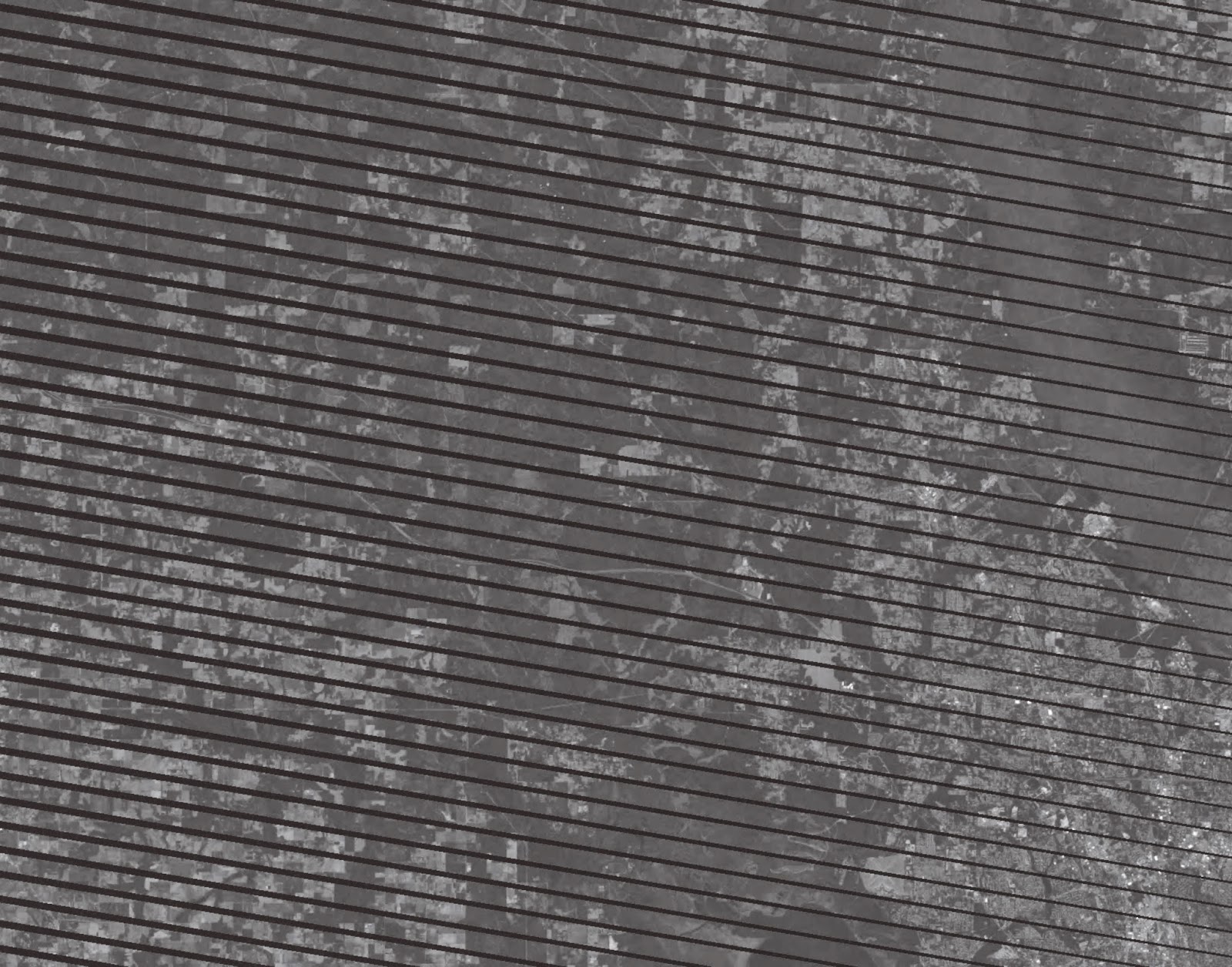
Image 1: This image is a JPEG version of the original .tif file used as the source data.

The image was supplied as a TIF file.  Using ArcCatalog, I was able to create a new shapefile and use the create features tool to digitize a variety of land use and land cover types, based on my understanding of photo interpretation so far.

A cursory examination suggests that there is a large tidal zone dominating the left side of the image.  This is likely a tidal zone due to the presence of tidal flats, and the sinuous quality of the channels.


There is a large road running through the middle right which appears to be a center of commercial activity.  This proximity influenced many of my categorizations of the parcels as "commercial services.

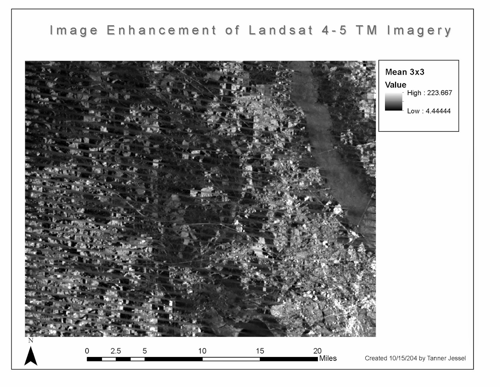
Map 1: Resulting graphic communicating my land cover and land use classifications.

 The final map included a neatline.  I would have preferred to somehow "clip" the edges of the shapefile to the graph.  

I felt confident in characterizing the following land uses and land covers:

• Industrial
• Residential
• Commercial Services
• Other Urban
• Streams and Canals
• Lake
• Bays and Estuaries
• Deciduous Forest Land
• Mixed Forest Land
• Nonforested Wetland
• Forested Wetland

The codes, description, features, and rationale for each of these areas is described in the table that follows.

Code	Description	Features	Decision Points
113	Industrial	Industrial. Large facilities, vehicles	Proximity away from residences, other commercial areas, equipment
111	Residential	Single Family Homes, Driveways, Lawns, School	Proximity to main throroughfare, commercial area, waterways
112	Commercial Services	Business	Proximity to main thoroughfare, parking lots, air conditioners
117	Other Urban	Cemetery	Headstones indicate cemetery
551	Streams and Canals	Linear waterway	Apart from main estuarine environment
552	Lake	Circular water feature	Dark tone, very fine texture, isolated
554	Bays and Estuaries	Large area, sinuous form, tidal areas	Dark tone, fine texture, to boundary of tidal areas.
441	Deciduous Forest Land	Trees of uniform consistency	Very coarse texture, homogenous, uniform color
443	Mixed Forest Land	Trees of varied consitency	Very coarse  texture, heterogenous, varied color
662	Nonforested Wetland	Vegetation and tidal flats of varied color	Fine texture, proximity to water, proximity to estuary
661	Forested Wetland	Shrubs of varied color	Coarse textture, proximity to water, estuary, river

GIS404 Remote Sensing - Module 3 Learning Objectives - Land Use Land Cover Classification

Topics Covered in Module 3:

• Land Use Land Cover (LULC) Classification
• Definitions of Land Use and Land Cover
• Reasons for LULC Classifications
• LULC Classification Process
• Geographic Extent of Study Classification (or Taxonomic) Scale and System (e.g. LULC types)
• Minimum Mapping Unit (MMU) and Spatial Resolution
• Visual (vs automated) Interpretation of Imagery
• Ground Truthing and Field Sampling
• Urban Imagery Resolution Requirements  (spatial, spectral, temporal)
• Accuracy Assessment
• Project Examples and Change Analysis
• Case Study and Products

Module 3 Learning Objectives:

• Recall the differences between Land Use and Land Cover
• Recall how hierarchical systems are used for Land Use and Land Cover (LULC) classification (e.g. USGS)
• Recall the process for implementing a Land Use and Land Cover classification 
• Recall how different types (e.g. Urban) of LULC classifications have different image requirements (e.g. resolution) as well as Minimum Mapping Units (MMU) 

Module 3 Learning Outcomes:

• Apply recognition elements to Land Use Land Cover (LULC) classification
• Identify various features using aerial photography
• Construct a land use / land cover map

GIS404 Remote Sensing - Module 2 Lab Assignments - Aerial Photography Basics & Visual Interpretation of Aerial Photography

I had made another one using a different method that I like somewhat better, in terms of labelling.

Map depicting layers within a single shapefile for areas of varying degrees of tone and texture.

Map depicting varying features identified from aerial photography based on ancillary cues from the image.

GIS404 Remote Sensing - Module 2 Learning Objectives - Aerial Photography Basics & Visual Interpretation of Aerial Photography

Module 2 Student Learning Outcomes

• Recall the major types of aerial photos/cameras
• Recall the types of films, resolution and products generally produced from aerial photos
• Recall case study examples of the visual interpretation of aerial photos
• Recall how to use various recognition elements to visually interpret aerial photographs
• Interpret the tone and texture of aerial photographs
• Identify land features in an aerial photograph based on several visual attributes
• Compare similar land features in true color and false color infrared (IR) photographs

By the end of this lab, you should be able to:

• Interpret the tone and texture of aerial photographs
• Identify land features in an aerial photograph based on several visual attributes
• Compare similar land features in true color and false color infrared (IR) photographs